Google Sheet Functions That Can Do More Than Just Maths

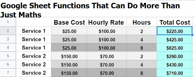
We all have used Google Sheets for many reasons. One can smoothly perform addition, subtraction, multiplication, average, and other mathematical operations, but Google Sheets has more potential than that. The users can do a lot more than just solving some mathematical problems. Google Sheets are widely used for professional work in big companies to save their data and segregate them properly. It helps the users in translation, which means one can easily translate a phrase in another language. Google Sheets provides a wide variety of languages to consumers. Hence one can select the language in which he/she wants to translate. It also helps to pull out the vital information from the web and allows you to perform formatting whenever required. So if you are a Google Sheet user, or want to learn more about the exciting features of it, this article is for you. So stay with us till the end.

Capitalization issue

Sometimes when users want to collect information from different sources, chances are the data do not have uniformity. Some words might be in upper cases while others in lower, and some might have a mixture of both. To correct that, and imagine if the data is in hundreds, one has to spend long hours, which is eventually not possible. Here Google Sheets ‘PROPER’ feature kicks in.

‘PROPER’ fixes the problem by reformatting the texts in Sheets. It ensures that all the text starts with a capital letter and followed by small letters. So it includes features like UPPER, LOWER, and TRIM. All these have their specific job to do in the Sheets.

UPPER changes the text into uppercase, LOWER changes the text into lowercase and TRIM deletes the unnecessary space between the text. So in this way, Google sheet solves the problem and provides uniformity to the data.

Translate

One may receive a Google sheet having the data of an unknown language. Now it would become impossible to understand the data and work on it. But Google Sheets has a solution for it. Google Sheet introduced the ‘GOOGLETRANSLATE’ function. The Translator translates a phrase or text in any preferred language. All one needs to do is command ‘GOOGLETRANSLATE’. The user can also choose language accordingly. For example, if one wants to change a phrase into Spanish in cell A2, all he/she needs to type is command ‘GOOGLETRANSLATE(A2, “fr”,”es”)’

The general syntax is: GOOGLETRANSLATE(text, [source_language, target_language])

where: text- is the text to translate

            source_language- is the text that is to be detected.

            target_language- is the text in which the data will translate

Since there are different languages available to change the text, one must learn the code of the language to give the command correctly, some of them are given below.

English(en), Spanish(es), Korean(ko), Japanese(ja), etcetera

One can also detect the language of the data. For example, if you receive any file with unknown language data, and you want to know which language is this, you can have easy access to that also. Google Sheet has the ‘DETECTLANGUAGE’ feature, which allows detecting any language.

IMPORTRANGE

Let’s say you want to share specific details from some spreadsheets but not the entire data. Or you want to grab some data out of another. You don’t want to involve everything that was in the original file. Here Google Sheet provides an IMPORTRANGE function. It provides a hassle-free job to its users. One can easily extract out the exact information from a preferred sheet or a cell. To do that, one needs to give a simple command, and the rest will be done quickly.

The syntax of the command can be followed as:

‘IMPORTRANGE (“spreadsheeturl”, “Sheetname!Cell_number1:Cell_number2”)’

where “spreadsheeturl” should be removed by the actual spreadsheet URL. And, the name of the sheet and the details must be according to the requirement.

IMPORTHTML and IMPORTFEED

One can also use IMPORTHTML and IMPORTFEED to gather information directly from the web. One needs to give the command IMPORTHTML or IMPORTFEED followed by the required link, and the Google Sheet will automatically do the rest.

For example, to gather a list of popular restaurants, the user needs to type

‘=IMPORTHTML( “https://en.wikipedia.org/wiki/List _of_popular_restaurants”, “table”, 3)’

And the Sheet will collect all the required data within a few seconds.

Or, to get updates about sports from the New York Times, type.

‘=IMPORTFEED( “link_of_the_website.”)’

Mini Chart

Google Sheets also provide a fantastic function called SPARKLINE. With this function, one can create a mini chart of the given data in the Sheet. And can easily track all the information accordingly. It also allows users to analyze the data by using SPARKLINE quickly. To use it, one needs to follow a command, and the spreadsheet will do the rest. One can also select which chart they want to put in like.

Syntax of command

‘=SPARKLINE(data, [options])’

where, data- the range containing data, and[optional]- which means you can customize the chart with the options mentioned below:

“Line”-  for line graph

“Bar”- for bar chart

“Column”-  column chart

“Xmin”- minimum x-axis

“Xmax”- maximum x-axis

“Color”- the color of the line, and etcetera

These are features you can use in your Google Sheet and can do your work effortlessly. You can share it with your friends to make their life easy. Try these tips and features, and you will like working on the spreadsheet. I hope this article was helpful.

SOURCE:- Google Sheet Functions That Can Do More Than Just Maths